Excitable Dynamics with mxlpy — The FitzHugh-Nagumo Model

The Hodgkin-Huxley model captures neuron dynamics with high biophysical fidelity, but four coupled ODEs with nonlinear voltage-dependent coefficients make it hard to reason about intuitively. In 1961, Richard FitzHugh reduced the essential mathematics to two variables, and in 1962 Jin-ichi Nagumo built an electronic circuit that implements the same equations. The result is the FitzHugh-Nagumo (FHN) model: the simplest system that captures excitability, threshold behaviour, and limit cycle oscillations.

It is widely used beyond neuroscience — the same structure appears in cardiac models, chemical oscillators, and pattern-forming systems.

The Model

Two variables:

• v — fast variable, analogous to membrane voltage
• w — slow variable, analogous to a recovery current

dv/dt = v  −  v³/3  −  w  +  I_ext
dw/dt = (v + a  −  b·w) / tau

Parameter	Role
I_ext	External drive — raises or lowers excitability
a, b	Shape of the w-nullcline
tau	Timescale separation — w is slow when tau is large

With a = 0.7, b = 0.8, tau = 12.5, I_ext = 0.5, the system oscillates continuously. With smaller I_ext, it is excitable: a perturbation triggers one spike before returning to rest.

import numpy as np
import matplotlib.pyplot as plt
from pathlib import Path
from mxlpy import Model, Simulator, fns

ASSETS = Path("dist/assets")
ASSETS.mkdir(parents=True, exist_ok=True)

time = np.linspace(0, 200, 4000)


# mxlpy requires named functions
def fhn_dv(v, w, I_ext):
    return v - v**3 / 3 - w + I_ext


def fhn_dw(v, w, a, b, tau):
    return (v + a - b * w) / tau


def fhn() -> Model:
    return (
        Model()
        .add_variables({"v": -1.2, "w": -0.6})
        .add_parameters({"a": 0.7, "b": 0.8, "tau": 12.5, "I_ext": 0.5})
        .add_reaction("dv", fn=fhn_dv, args=["v", "w", "I_ext"], stoichiometry={"v": 1})
        .add_reaction(
            "dw", fn=fhn_dw, args=["v", "w", "a", "b", "tau"], stoichiometry={"w": 1}
        )
    )

With stoichiometry={'v': 1}, mxlpy sets dv/dt = rate × 1 = fhn_dv(v, w, I_ext). This works for any ODE right-hand side we can express as a named function — not just mass-action kinetics.

variables, fluxes = (
    Simulator(fhn()).simulate_time_course(time).get_result().unwrap_or_err()
)

fig_tc, ax = plt.subplots(figsize=(9, 3))
variables[["v", "w"]].plot(ax=ax)
ax.set_xlabel("Time")
ax.set_title("FitzHugh-Nagumo: time course")
plt.tight_layout()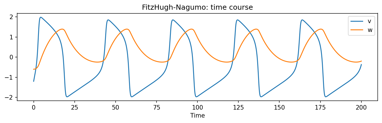

v fires in fast spikes; w follows slowly, acting as a brake that prevents the system from staying depolarised. The large timescale separation (tau = 12.5) is what gives the spikes their sharp upstroke and slow recovery.

Phase Plane Analysis

The most illuminating view of a two-variable system is the phase plane: plot v against w and overlay the nullclines — the curves where each derivative is zero.

• v-nullcline (dv/dt = 0): w = v − v³/3 + I_ext — cubic, N-shaped
• w-nullcline (dw/dt = 0): w = (v + a) / b — straight line

The intersection is the equilibrium. When it lies on the middle branch of the cubic (the unstable branch), the system has no stable fixed point and oscillates — a limit cycle.

v_range = np.linspace(-2.5, 2.5, 400)
v_nc = v_range - v_range**3 / 3 + 0.5  # v-nullcline: w = v - v^3/3 + I
w_nc = (v_range + 0.7) / 0.8  # w-nullcline: w = (v + a) / b

fig_ph, ax = plt.subplots(figsize=(6, 6))
ax.plot(v_range, v_nc, label="v-nullcline (dv/dt = 0)", color="tab:blue")
ax.plot(v_range, w_nc, label="w-nullcline (dw/dt = 0)", color="tab:orange")
ax.plot(
    variables["v"],
    variables["w"],
    color="gray",
    linewidth=0.8,
    alpha=0.8,
    label="trajectory",
)
ax.set_xlim(-2.5, 2.5)
ax.set_ylim(-1.0, 2.0)
ax.set_xlabel("v")
ax.set_ylabel("w")
ax.set_title("FitzHugh-Nagumo: phase plane")
ax.legend()
plt.tight_layout()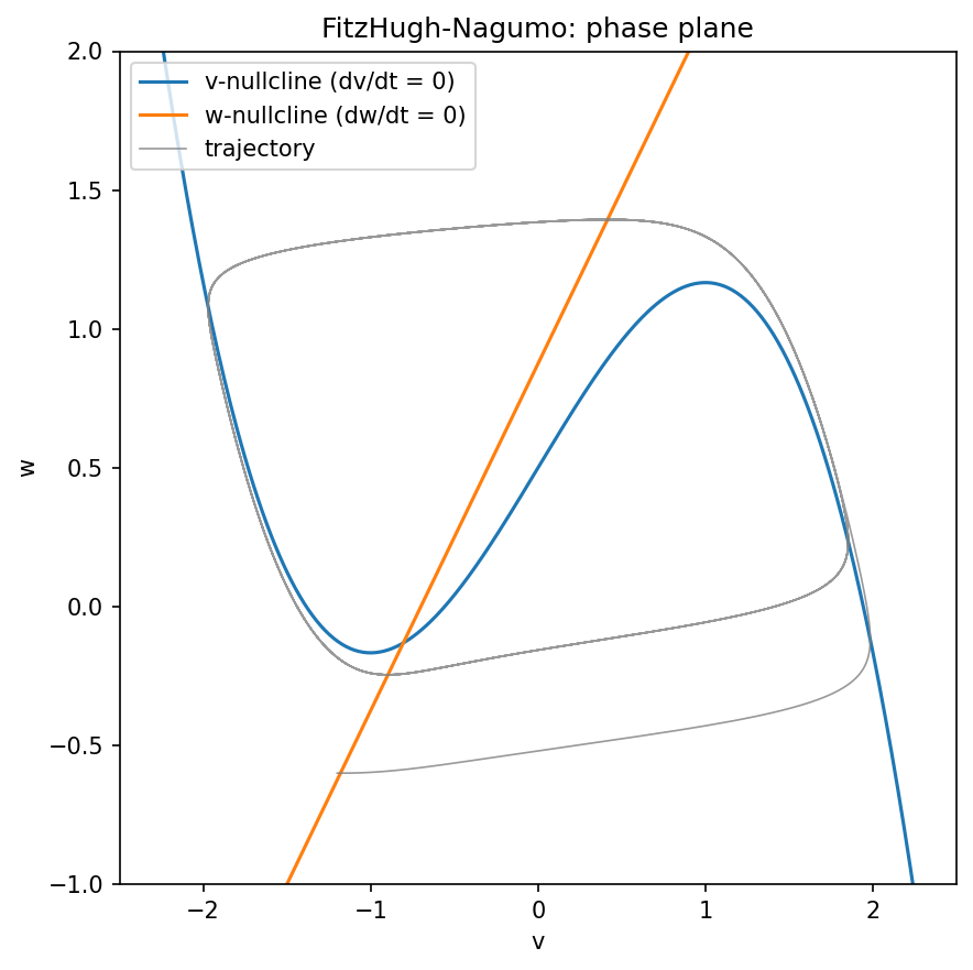

The trajectory circles around the intersection of the two nullclines. Because that intersection sits on the middle (unstable) branch of the cubic, no stable fixed point exists and the system settles onto a limit cycle — a closed orbit that attracts all nearby trajectories.

What’s Next

• Reduce I_ext below the Hopf bifurcation (~0.34) — the system should become excitable rather than oscillatory.
• Vary tau to see how timescale separation affects spike shape.
• The models so far have all been in biology or neuroscience. In the next post we apply the same mxlpy workflow to a model from economics: the Solow-Swan growth model.