The Hodgkin-Huxley Model — Action Potentials from First Principles

In 1952, Alan Hodgkin and Andrew Huxley published a quantitative description of how the squid giant axon generates an action potential. Their model earned them the Nobel Prize in 1963 and remains the foundation of computational neuroscience today.

The core insight is that the neuron membrane acts like a capacitor charged by ion currents through voltage-gated channels. The channels open and close in a voltage-dependent way, described by gating variables that follow their own ODEs. The result is a four-dimensional system that produces the characteristic spike shape of an action potential.

The Model

Four state variables:

Variable	Meaning
V	Membrane potential (mV)
m	Na⁺ channel activation gate
h	Na⁺ channel inactivation gate
n	K⁺ channel activation gate

The membrane voltage ODE (divided by capacitance C_m):

C_m · dV/dt = I_ext  −  g_Na · m³ · h · (V − E_Na)
                     −  g_K  · n⁴ · (V − E_K)
                     −  g_L  · (V − E_L)

Each gating variable x ∈ {m, h, n} follows:

dx/dt = α_x(V) · (1 − x)  −  β_x(V) · x

where α_x and β_x are empirical voltage-dependent rate constants fit by Hodgkin and Huxley to their voltage-clamp data.

import numpy as np
import matplotlib.pyplot as plt
from pathlib import Path
from mxlpy import Model, Simulator, fns

ASSETS = Path("dist/assets")
ASSETS.mkdir(parents=True, exist_ok=True)

time = np.linspace(0, 100, 10000)  # 100 ms

Rate functions

The α and β functions have singularities that we handle explicitly. mxlpy requires named functions (no lambdas), so we define them at module level.

# Hodgkin-Huxley alpha/beta functions
def _alpha_m(v):
    return 1.0 if abs(v + 40) < 1e-7 else 0.1 * (v + 40) / (1 - np.exp(-(v + 40) / 10))


def _beta_m(v):
    return 4.0 * np.exp(-(v + 65) / 18)


def _alpha_h(v):
    return 0.07 * np.exp(-(v + 65) / 20)


def _beta_h(v):
    return 1.0 / (1 + np.exp(-(v + 35) / 10))


def _alpha_n(v):
    return 0.1 if abs(v + 55) < 1e-7 else 0.01 * (v + 55) / (1 - np.exp(-(v + 55) / 10))


def _beta_n(v):
    return 0.125 * np.exp(-(v + 65) / 80)


# mxlpy reaction rate functions — currents divided by C_m
def i_na_rate(g_na, m, h, v, e_na, c_m):
    return g_na * m**3 * h * (v - e_na) / c_m


def i_k_rate(g_k, n, v, e_k, c_m):
    return g_k * n**4 * (v - e_k) / c_m


def i_l_rate(g_l, v, e_l, c_m):
    return g_l * (v - e_l) / c_m


def i_ext_rate(i_ext, c_m):
    return i_ext / c_m


# Gating variable kinetics
def m_act(v, m):
    return _alpha_m(v) * (1 - m)


def m_inact(v, m):
    return _beta_m(v) * m


def h_act(v, h):
    return _alpha_h(v) * (1 - h)


def h_inact(v, h):
    return _beta_h(v) * h


def n_act(v, n):
    return _alpha_n(v) * (1 - n)


def n_inact(v, n):
    return _beta_n(v) * n

def hodgkin_huxley() -> Model:
    # Steady-state gating variables at resting potential
    v0 = -65.0
    m0 = _alpha_m(v0) / (_alpha_m(v0) + _beta_m(v0))
    h0 = _alpha_h(v0) / (_alpha_h(v0) + _beta_h(v0))
    n0 = _alpha_n(v0) / (_alpha_n(v0) + _beta_n(v0))

    return (
        Model()
        .add_variables({"V": v0, "m": m0, "h": h0, "n": n0})
        .add_parameters(
            {
                "C_m": 1.0,  # uF/cm²
                "g_Na": 120.0,
                "g_K": 36.0,
                "g_L": 0.3,  # mS/cm²
                "E_Na": 50.0,
                "E_K": -77.0,
                "E_L": -54.4,  # mV
                "I_ext": 10.0,  # uA/cm²
            }
        )
        # Membrane voltage (stoichiometry ±1; rate already divided by C_m)
        .add_reaction(
            "I_Na",
            fn=i_na_rate,
            args=["g_Na", "m", "h", "V", "E_Na", "C_m"],
            stoichiometry={"V": -1},
        )
        .add_reaction(
            "I_K",
            fn=i_k_rate,
            args=["g_K", "n", "V", "E_K", "C_m"],
            stoichiometry={"V": -1},
        )
        .add_reaction(
            "I_L", fn=i_l_rate, args=["g_L", "V", "E_L", "C_m"], stoichiometry={"V": -1}
        )
        .add_reaction(
            "v1", fn=i_ext_rate, args=["I_ext", "C_m"], stoichiometry={"V": 1}
        )
        # Gating variables
        .add_reaction("m_act", fn=m_act, args=["V", "m"], stoichiometry={"m": 1})
        .add_reaction("m_inact", fn=m_inact, args=["V", "m"], stoichiometry={"m": -1})
        .add_reaction("h_act", fn=h_act, args=["V", "h"], stoichiometry={"h": 1})
        .add_reaction("h_inact", fn=h_inact, args=["V", "h"], stoichiometry={"h": -1})
        .add_reaction("n_act", fn=n_act, args=["V", "n"], stoichiometry={"n": 1})
        .add_reaction("n_inact", fn=n_inact, args=["V", "n"], stoichiometry={"n": -1})
    )

Each gating variable is split into two reactions: one that opens the gate (act) and one that closes it (inact). The net rate is their difference, which is exactly dx/dt = α(V)·(1−x) − β(V)·x.

variables, fluxes = (
    Simulator(hodgkin_huxley()).simulate_time_course(time).get_result().unwrap_or_err()
)

fig_v, ax = plt.subplots(figsize=(9, 3))
variables["V"].plot(ax=ax, color="tab:blue")
ax.set_xlabel("Time (ms)")
ax.set_ylabel("Membrane potential (mV)")
ax.set_title("Hodgkin-Huxley: action potentials")
plt.tight_layout()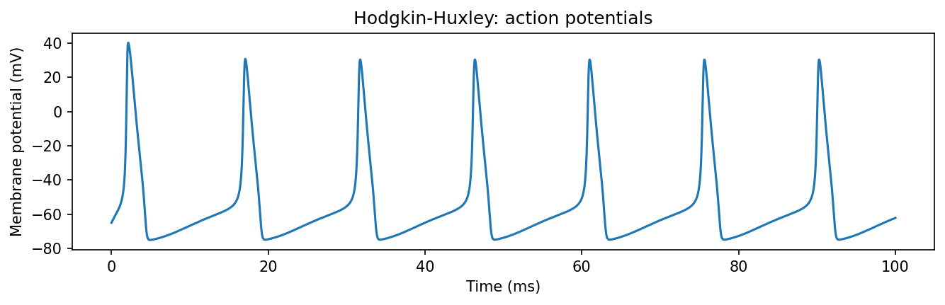

With I_ext = 10 µA/cm², the neuron fires repetitively. Each spike is about 100 mV tall and lasts roughly 1 ms — matching experimental recordings from the squid axon.

Gating Variables

The shape of each action potential is determined by the relative timing of the three gates:

• m (Na⁺ activation): opens fast when V depolarises → drives the upstroke
• h (Na⁺ inactivation): closes slowly after activation → terminates Na⁺ current
• n (K⁺ activation): opens slowly → drives repolarisation and undershoot

fig_g, axes = plt.subplots(3, 1, figsize=(9, 6), sharex=True)

for ax, (gate, color, label) in zip(
    axes,
    [
        ("m", "tab:orange", "m  (Na activation)"),
        ("h", "tab:red", "h  (Na inactivation)"),
        ("n", "tab:green", "n  (K activation)"),
    ],
):
    variables[gate].plot(ax=ax, color=color)
    ax.set_ylabel(label)
    ax.set_ylim(-0.05, 1.05)

axes[-1].set_xlabel("Time (ms)")
fig_g.suptitle("Hodgkin-Huxley: gating variables")
plt.tight_layout()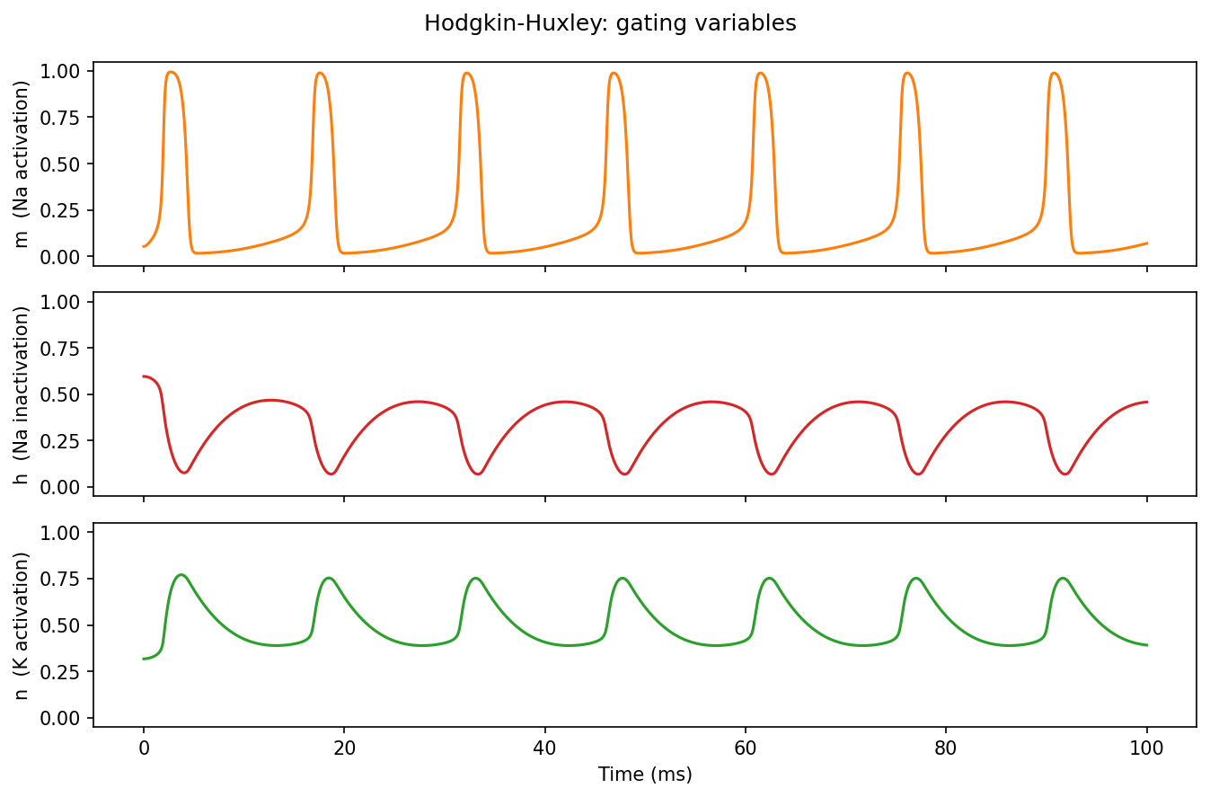

During each spike: m jumps up fast (Na⁺ influx, upstroke), h falls slowly (Na⁺ channel inactivation, peak termination), and n rises slowly (K⁺ efflux, repolarisation). Between spikes, all three gates return toward their resting values — h recovers last, which is why there is a refractory period.

What’s Next

• Lower I_ext toward the firing threshold (~6.5 µA/cm²) to see the transition from silence to spiking.
• Clamp I_ext = 0 and give a brief current pulse — the model produces a single action potential, then returns to rest.
• The Hodgkin-Huxley model is biophysically detailed but expensive to simulate. In the next post we look at the FitzHugh-Nagumo model: a two-variable reduction that captures the essential spike dynamics at a fraction of the complexity.