Enzymatic Chains with mxlpy — Linear Michaelis-Menten Kinetics

Many metabolic pathways are linear sequences of enzymatic reactions: substrate S1 is converted to S2, then to S3, and so on. Each step follows Michaelis-Menten kinetics — the rate saturates at high substrate concentrations and is half-maximal when the substrate equals the Michaelis constant K_m.

This post builds an n-step chain programmatically in mxlpy. The point is not the biology — it is to show that mxlpy lets you build models with loops and parameters, not just by hand.

The Model

An n-step chain has n substrates S1, S2, …, Sn and n−1 reactions:

S1  →  S2  →  S3  →  …  →  Sn

Each reaction follows Michaelis-Menten kinetics:

v_i = Vmax_i · S_i / (Km_i + S_i)

mxlpy provides fns.michaelis_menten_1s(s, vmax, km) as a built-in rate function, so no custom functions are needed here.

The model factory below generates a chain of any length.

import numpy as np
import matplotlib.pyplot as plt
from pathlib import Path
from mxlpy import Model, Simulator, fns

ASSETS = Path("dist/assets")
ASSETS.mkdir(parents=True, exist_ok=True)

time = np.linspace(0, 15, 1000)


def linear_mm(n_steps: int = 4) -> Model:
    model = Model()
    model.add_variables(
        {f"S{i}": (1.0 if i == 1 else 0.0) for i in range(1, n_steps + 1)}
    )
    model.add_parameters(
        {f"Vmax{i}": 1.0 for i in range(1, n_steps)}
        | {f"Km{i}": 0.3 for i in range(1, n_steps)}
    )
    for i in range(1, n_steps):
        model.add_reaction(
            f"v{i}",
            fn=fns.michaelis_menten_1s,
            args=[f"S{i}", f"Vmax{i}", f"Km{i}"],
            stoichiometry={f"S{i}": -1, f"S{i + 1}": 1},
        )
    return model

The factory works because mxlpy’s add_variables, add_parameters, and add_reaction all accept dynamic names. The model structure is programmatically generated — adding another step requires only changing n_steps.

variables, fluxes = (
    Simulator(linear_mm(n_steps=5))
    .simulate_time_course(time)
    .get_result()
    .unwrap_or_err()
)

fig_tc, ax = plt.subplots(figsize=(8, 4))
variables.plot(ax=ax)
ax.set_xlabel("Time")
ax.set_ylabel("Concentration")
ax.set_title("Linear MM chain (5 steps): substrate time courses")
plt.tight_layout()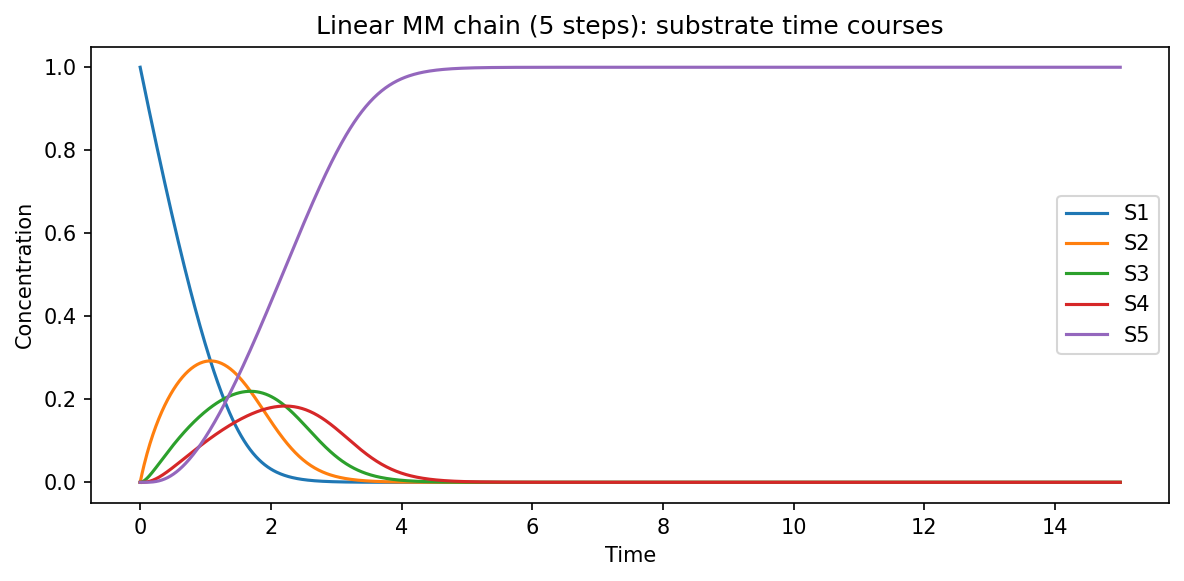

S1 drains first, filling S2, which in turn fills S3, and so on. Each substrate peaks later than the one before it. At steady state, all reaction rates are equal — flux is conserved along the chain.

Signal Delay vs Chain Length

Longer chains delay the appearance of the final product. We can quantify this by tracking when the last substrate S_n reaches its half-maximum concentration as a function of chain length.

time_long = np.linspace(0, 30, 2000)
chain_lengths = [2, 3, 4, 5, 6, 7]

fig_cmp, ax = plt.subplots(figsize=(8, 4))

for n in chain_lengths:
    variables, _ = (
        Simulator(linear_mm(n_steps=n))
        .simulate_time_course(time_long)
        .get_result()
        .unwrap_or_err()
    )
    variables[f"S{n}"].plot(ax=ax, label=f"n = {n}")

ax.set_xlabel("Time")
ax.set_ylabel(f"Final substrate S_n")
ax.set_title("Signal delay grows with chain length")
ax.legend()
plt.tight_layout()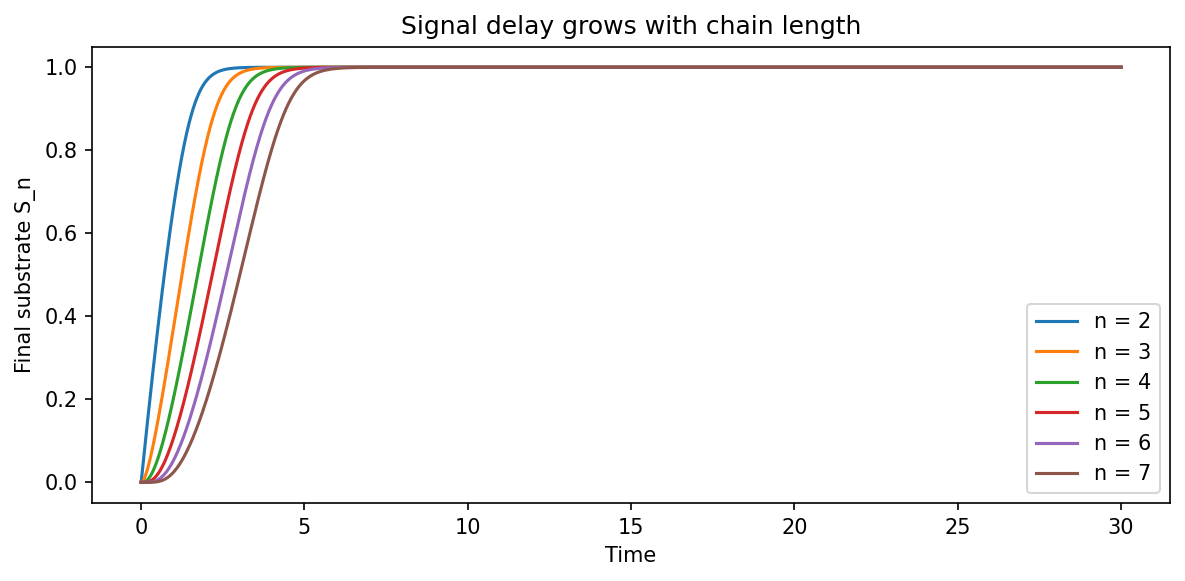

The final product accumulates progressively later as the chain grows. This is a direct consequence of the serial nature of the reactions — each substrate must fill before the next can begin to be produced. Cells exploit this property to create temporal delays in signalling cascades.

What’s Next

• Vary Km along the chain — how does a bottleneck step (high Km, low Vmax) affect the overall flux?
• Add feedback inhibition: let the final product S_n inhibit the first reaction. This is a common regulatory motif in amino acid biosynthesis.
• In a future post we will use mxlpy’s parameter estimation tools to fit Vmax and Km values to time-course data.