Predator-Prey Cycles with mxlpy — The Lotka-Volterra Model

In the 1920s Alfred Lotka and Vito Volterra independently derived the same pair of equations describing how predator and prey populations drive each other’s oscillations. Their model is surprisingly accurate: fur-trade records from the Hudson’s Bay Company spanning a century show hare and lynx populations cycling with a period and shape that match the equations closely.

We will build this model in mxlpy and explore its two characteristic features: periodic oscillations in time, and closed orbits in phase space.

The Model

Two populations: H (prey, e.g. hares) and L (predators, e.g. lynx). Four events drive the dynamics:

Reaction	Rate	Effect
Prey reproduce	alpha · H	H +1
Prey are eaten	beta · H · L	H −1
Predators grow from eating	delta · H · L	L +1
Predators die	gamma · L	L −1

The ODEs that follow:

dH/dt =  alpha · H  −  beta · H · L
dL/dt =  delta · H · L  −  gamma · L

Predation and predator growth share the same functional form (H · L) but different rate constants — beta sets how fast prey die, delta sets how efficiently that converts to predator growth.

import numpy as np
import matplotlib.pyplot as plt
from pathlib import Path
from mxlpy import Model, Simulator, fns

ASSETS = Path("dist/assets")
ASSETS.mkdir(parents=True, exist_ok=True)

time = np.linspace(0, 40, 2000)

def lv() -> Model:
    return (
        Model()
        .add_variables({"H": 10.0, "L": 5.0})
        .add_parameters({"alpha": 1.0, "beta": 0.1, "delta": 0.075, "gamma": 1.5})
        .add_reaction(
            "prey_birth",
            fn=fns.mass_action_1s,
            args=["alpha", "H"],
            stoichiometry={"H": 1},
        )
        .add_reaction(
            "predation",
            fn=fns.mass_action_2s,
            args=["beta", "H", "L"],
            stoichiometry={"H": -1},
        )
        .add_reaction(
            "predator_growth",
            fn=fns.mass_action_2s,
            args=["delta", "H", "L"],
            stoichiometry={"L": 1},
        )
        .add_reaction(
            "predator_death",
            fn=fns.mass_action_1s,
            args=["gamma", "L"],
            stoichiometry={"L": -1},
        )
    )

Predation and predator growth are two separate reactions with the same rate law but different parameters and stoichiometries. mxlpy tracks the flux through each process independently — useful when we later want to ask ‘how much prey is consumed per unit time?’

variables, fluxes = (
    Simulator(lv()).simulate_time_course(time).get_result().unwrap_or_err()
)

fig_tc, ax = plt.subplots(figsize=(8, 4))
variables.plot(ax=ax)
ax.set_xlabel("Time")
ax.set_ylabel("Population")
ax.set_title("Lotka-Volterra: time course")
plt.tight_layout()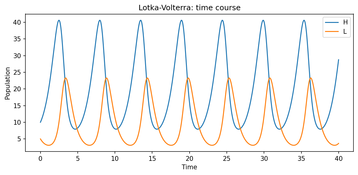

Both populations oscillate with a fixed period. The predator peak always lags behind the prey peak: prey grows first, predators follow, prey collapses under predation pressure, predators starve, and the cycle repeats.

Phase Portrait

Instead of watching H and L evolve over time, we can plot one against the other. Each point in this phase plane represents the complete state of the system at one instant. Because the classical Lotka-Volterra model conserves a quantity analogous to energy, trajectories are closed orbits — the system returns exactly to its starting point every cycle.

fig_ph, ax = plt.subplots(figsize=(5, 5))
ax.plot(variables["H"], variables["L"], color="steelblue", linewidth=1)
ax.plot(
    variables["H"].iloc[0],
    variables["L"].iloc[0],
    "o",
    color="steelblue",
    label="start",
)
ax.set_xlabel("Prey (H)")
ax.set_ylabel("Predator (L)")
ax.set_title("Lotka-Volterra: phase portrait")
ax.legend()
plt.tight_layout()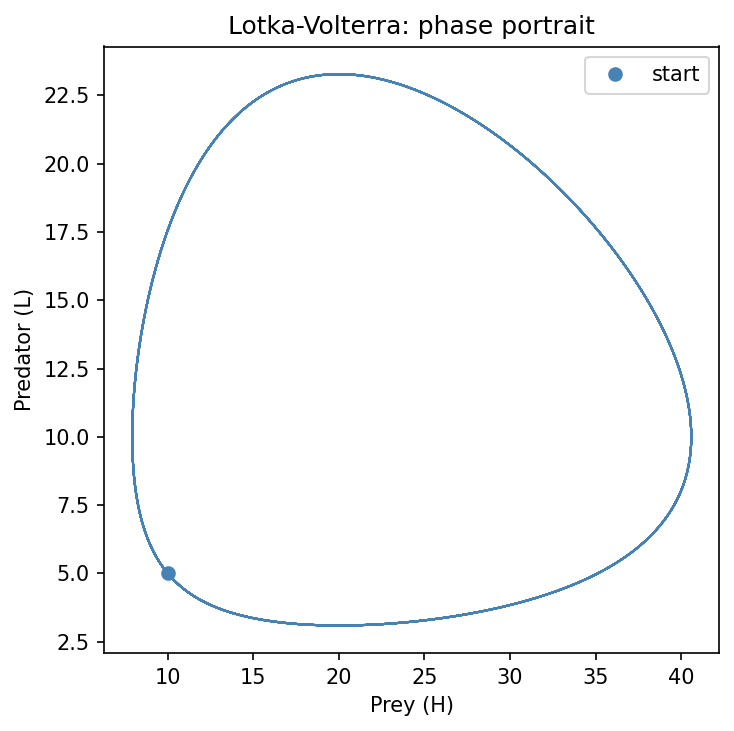

The closed loop confirms the system is periodic and conservative. Different starting points trace different orbits — always closed, never spiralling inward or outward. This structural property disappears as soon as we add realistic features like a carrying capacity for prey or predator saturation, which we will explore in a future post.

What’s Next

• Add a carrying capacity for prey: replace alpha · H with alpha · H · (1 − H/K). The orbit will spiral inward to a stable equilibrium.
• Start at the fixed point H* = gamma/delta, L* = alpha/beta — the system should stay there indefinitely.
• In the next post we step up in complexity: the Hodgkin-Huxley model, which uses a similar reaction structure to describe the electrical dynamics of a single neuron.