Building Epidemic Models with mxlpy — From SIR to SEIR Without Starting Over

Compartmental epidemic models are one of the oldest and most widely used tools in public health. The core idea is simple: divide a population into groups — compartments — and write down rules for how people move between them. Despite their simplicity, these models powered pandemic response decisions during COVID-19, influenza outbreaks, and many others.

In this post we will build a family of these models using mxlpy. The point is not just to simulate an epidemic — it is to show how mxlpy lets you start with a simple model and extend it incrementally, without ever rewriting the core from scratch.

The SIR Model

The simplest compartmental model splits a population into three groups:

• S — Susceptible (can catch the disease)
• I — Infected (currently sick and infectious)
• R — Recovered (immune, no longer infectious)

The population flows in one direction: S → I → R.

Two parameters control the dynamics:

Parameter	Meaning
beta	Transmission rate — how often a susceptible person becomes infected per contact with an infected person
gamma	Recovery rate — fraction of infected people who recover per unit time

The corresponding ODEs are:

dS/dt = -beta * S * I
dI/dt =  beta * S * I - gamma * I
dR/dt =  gamma * I

Building SIR in mxlpy

import numpy as np
import matplotlib.pyplot as plt
from pathlib import Path
from mxlpy import Model, Simulator, fns

ASSETS = Path("dist/assets")
ASSETS.mkdir(parents=True, exist_ok=True)

time = np.linspace(0, 200, 500)

def sir() -> Model:
    return (
        Model()
        .add_variables({"S": 0.99, "I": 0.01, "R": 0.0})
        .add_parameters({"beta": 0.3, "gamma": 0.05})
        .add_reaction(
            "infection",
            fn=fns.mass_action_2s,
            args=["beta", "S", "I"],
            stoichiometry={"S": -1, "I": 1},
        )
        .add_reaction(
            "recovery",
            fn=fns.mass_action_1s,
            args=["gamma", "I"],
            stoichiometry={"I": -1, "R": 1},
        )
    )

A few things to note about the mxlpy API:

• Fluent builder pattern — every .add_* call returns the model itself, so you can chain them.
• stoichiometry maps variable names to the sign of their change. {"S": -1, "I": 1} means: one unit leaves S, one unit enters I.
• Rate functions come from mxlpy.fns. mass_action_2s(k, s1, s2) evaluates to k * s1 * s2, which gives us beta * S * I.

Simulating and Plotting

variables, fluxes = (
    Simulator(sir()).simulate_time_course(time).get_result().unwrap_or_err()
)

fig_sir, ax = plt.subplots(figsize=(8, 4))
variables.plot(ax=ax)
ax.set_xlabel("Time (days)")
ax.set_ylabel("Fraction of population")
ax.set_title("SIR model")
plt.tight_layout()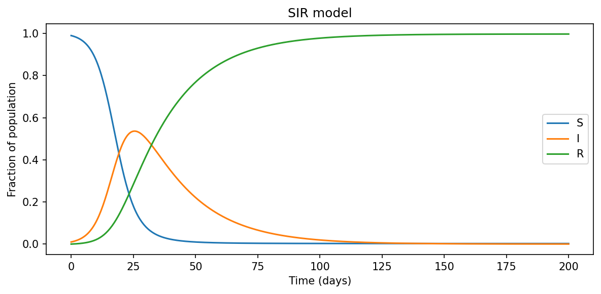

You should see the classic epidemic curve: a wave of infections that rises, peaks, and declines as susceptibles run out and recoveries accumulate.

---

Extending to SIRD — Adding Disease-Induced Mortality

The SIR model assumes everyone recovers. That is often a reasonable simplification, but sometimes we want to track deaths explicitly. The SIRD model adds a D (Deceased) compartment. Infected individuals now either recover or die:

dS/dt = -beta * S * I
dI/dt =  beta * S * I - gamma * I - mu * I
dR/dt =  gamma * I
dD/dt =  mu * I

Here mu is the disease-induced mortality rate.

Extending the SIR Model

Here is the key insight: we do not rewrite the SIR model. We take the existing model and add what is new.

def sird() -> Model:
    return (
        sir()  # start from SIR
        .add_variable("D", 0.0)  # new compartment
        .add_parameter("mu", 0.005)  # mortality rate
        .add_reaction(
            "death",
            fn=fns.mass_action_1s,
            args=["mu", "I"],
            stoichiometry={"I": -1, "D": 1},
        )
    )

Three lines extend a model that took twelve to write. The infection and recovery dynamics are inherited unchanged. This is the composability that mxlpy is designed for.

variables, fluxes = (
    Simulator(sird()).simulate_time_course(time).get_result().unwrap_or_err()
)

fig_sird, ax = plt.subplots(figsize=(8, 4))
variables.plot(ax=ax)
ax.set_xlabel("Time (days)")
ax.set_ylabel("Fraction of population")
ax.set_title("SIRD model")
plt.tight_layout()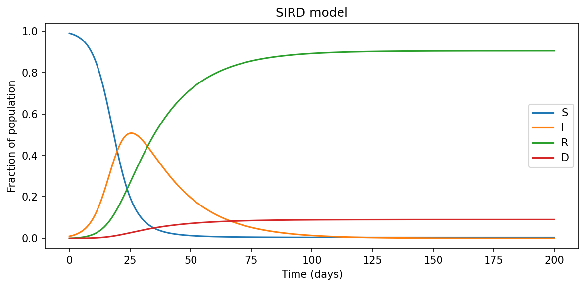

Notice how the recovered population is now slightly lower and the deceased compartment fills in — a small but meaningful distinction for policy planning.

---

Extending to SEIR — Adding an Incubation Period

Many diseases have an incubation period: infected individuals are not immediately infectious. The SEIR model captures this with an E (Exposed) compartment. Susceptibles first become exposed, then move to infectious:

dS/dt = -beta * S * I
dE/dt =  beta * S * I - sigma * E
dI/dt =  sigma * E - gamma * I
dR/dt =  gamma * I

sigma is the rate of progression from exposed to infectious (1/sigma = mean incubation period).

Extending SIR Again

We go back to the clean SIR model and extend in a different direction.

def seir() -> Model:
    return (
        sir()  # start from SIR
        .add_variable("E", 0.0)  # exposed compartment
        .add_parameter("sigma", 0.1)  # incubation rate
        .update_reaction(
            "infection",
            fn=fns.mass_action_2s,
            args=["beta", "S", "I"],
            stoichiometry={"S": -1, "E": 1},  # now S → E, not S → I
        )
        .add_reaction(
            "progression",
            fn=fns.mass_action_1s,
            args=["sigma", "E"],
            stoichiometry={"E": -1, "I": 1},
        )
    )

.update_reaction() changes only the stoichiometry of the existing infection reaction — the rate law (beta * S * I) is untouched. Exposed individuals then progress to infectious at rate sigma.

variables, fluxes = (
    Simulator(seir()).simulate_time_course(time).get_result().unwrap_or_err()
)

fig_seir, ax = plt.subplots(figsize=(8, 4))
variables.plot(ax=ax)
ax.set_xlabel("Time (days)")
ax.set_ylabel("Fraction of population")
ax.set_title("SEIR model")
plt.tight_layout()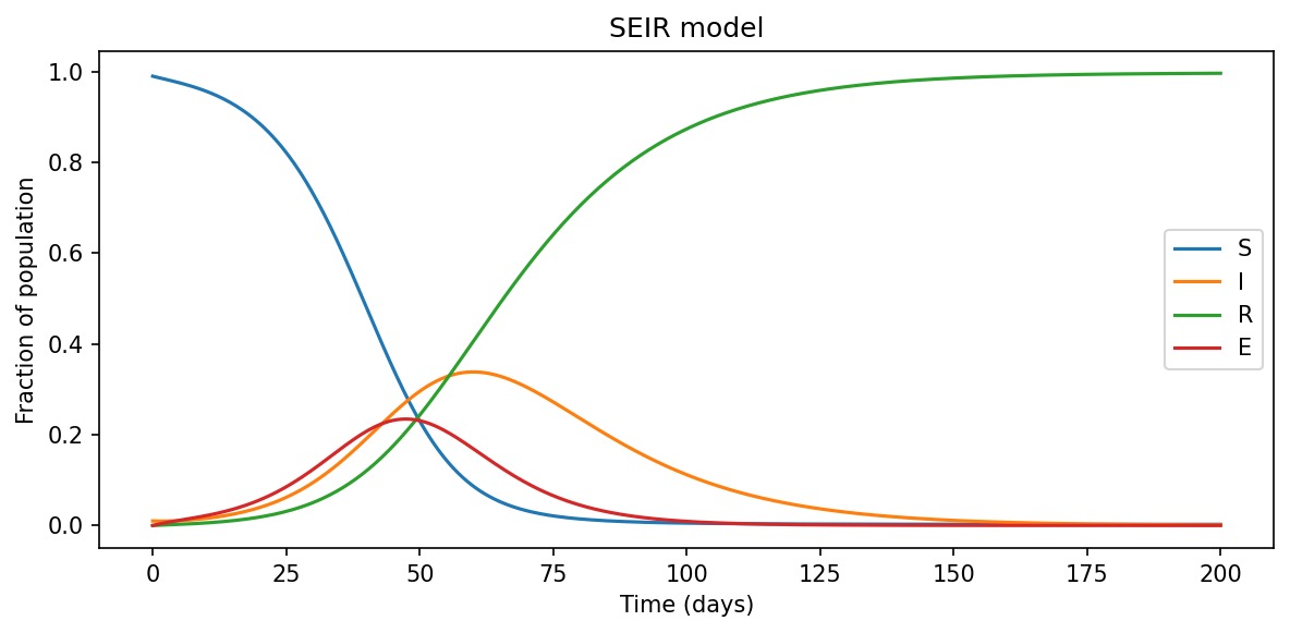

Compared to SIR, the SEIR epidemic peak is delayed and slightly smoothed out — a direct consequence of the incubation lag.

---

Comparing All Three Side by Side

One practical benefit of building models this way is that all three share the same interface. We can loop over them:

models = {"SIR": sir(), "SIRD": sird(), "SEIR": seir()}

fig_cmp, axes = plt.subplots(1, 3, figsize=(14, 4), sharey=True)

for ax, (name, model) in zip(axes, models.items()):
    variables, _ = (
        Simulator(model).simulate_time_course(time).get_result().unwrap_or_err()
    )
    variables["I"].plot(ax=ax, color="tab:red")
    ax.set_title(name)
    ax.set_xlabel("Time (days)")

axes[0].set_ylabel("Fraction infectious")
plt.tight_layout()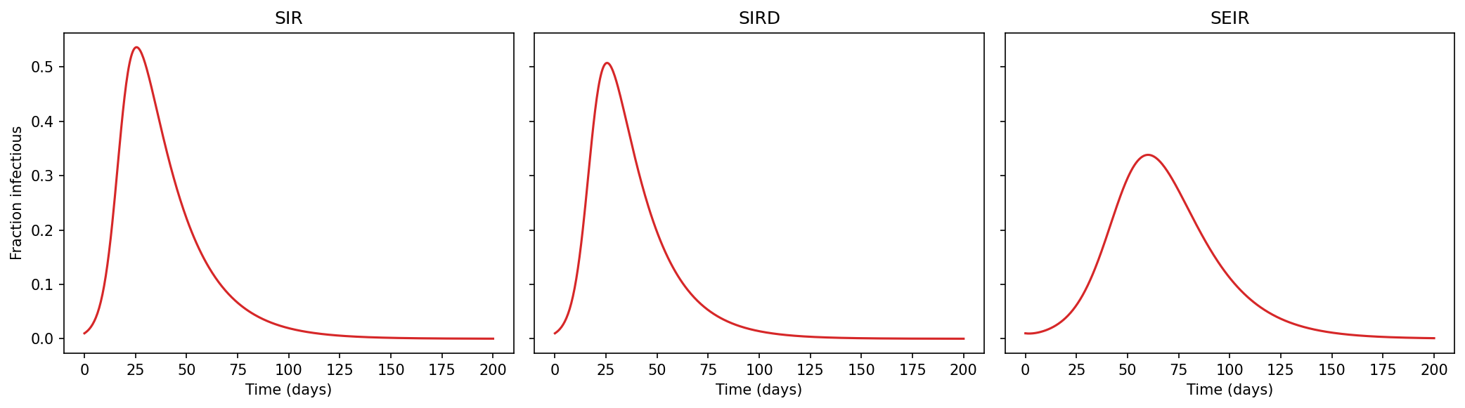

---

What Did We Actually Do?

We built three epidemiological models. More importantly, we built them as a family:

• SIR is the core — defined once, cleanly.
• SIRD extends SIR by adding a mortality branch.
• SEIR extends SIR by inserting an incubation stage.

Neither extension required touching the shared logic. In a traditional script-based workflow you would copy-paste the equations and risk introducing inconsistencies. Here, the shared structure is inherited and the differences are explicit.

This is the pattern mxlpy encourages throughout: define the simplest correct version, then extend rather than rewrite.

---

Next Steps

• Try combining the extensions: build a SEIRD model (incubation + mortality) by extending seir().
• Vary beta and gamma to explore the basic reproduction number R₀ = beta / gamma and its role in determining whether an epidemic takes off.
• In a future post we will fit these parameters to real outbreak data using mxlpy’s parameter estimation tools.