Economic Growth as an ODE — The Solow-Swan Model

The models we have built so far describe biological systems, but ODEs appear wherever quantities change continuously over time. In 1956, Robert Solow and Trevor Swan independently published a model of long-run economic growth that is structurally identical to the kinetic models we have been writing. It won Solow the Nobel Prize in 1987 and remains the starting point for macroeconomic growth theory.

The central question: given that an economy saves a fraction of its output and reinvests it as capital, and that capital depreciates over time, what is the long-run level of capital per worker?

The Model

One state variable: k, capital per effective worker.

Output per worker follows a Cobb-Douglas production function: y = k^alpha, where alpha ∈ (0,1) is the capital share of income.

Capital evolves as:

dk/dt = s · k^alpha  −  (delta + n) · k

Parameter	Meaning
s	Savings rate (fraction of output reinvested)
alpha	Capital elasticity of output
delta	Depreciation rate of capital
n	Population (labour force) growth rate

The steady state k* is where investment equals depreciation:

k* = (s / (delta + n))^(1 / (1 - alpha))

From any starting capital, the economy converges to k* — neither growing without limit nor collapsing to zero.

import numpy as np
import matplotlib.pyplot as plt
from pathlib import Path
from mxlpy import Model, Simulator, fns

ASSETS = Path("dist/assets")
ASSETS.mkdir(parents=True, exist_ok=True)

time = np.linspace(0, 200, 1000)


# Custom rate functions
def investment_rate(s, k, alpha):
    return s * k**alpha


def depreciation_rate(delta, n, k):
    return (delta + n) * k


def solow_swan() -> Model:
    return (
        Model()
        .add_variables({"k": 1.0})
        .add_parameters({"s": 0.3, "alpha": 0.3, "delta": 0.05, "n": 0.02})
        .add_reaction(
            "investment",
            fn=investment_rate,
            args=["s", "k", "alpha"],
            stoichiometry={"k": 1},
        )
        .add_reaction(
            "depreciation",
            fn=depreciation_rate,
            args=["delta", "n", "k"],
            stoichiometry={"k": -1},
        )
    )

# Compare convergence from different starting points
k_star = (0.3 / (0.05 + 0.02)) ** (1 / (1 - 0.3))

fig_tc, ax = plt.subplots(figsize=(8, 4))

for k0, color in [(0.5, "tab:blue"), (3.0, "tab:orange"), (15.0, "tab:green")]:
    variables, _ = (
        Simulator(solow_swan(), y0={"k": k0})
        .simulate_time_course(time)
        .get_result()
        .unwrap_or_err()
    )
    variables["k"].plot(ax=ax, color=color, label=f"k0 = {k0}")

ax.axhline(
    k_star, color="black", linestyle="--", linewidth=1, label=f"k* = {k_star:.1f}"
)
ax.set_xlabel("Time (years)")
ax.set_ylabel("Capital per worker k")
ax.set_title("Solow-Swan: convergence to steady state")
ax.legend()
plt.tight_layout()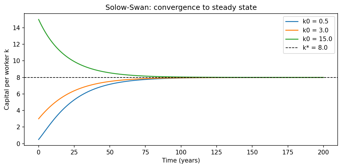

All three trajectories converge to the same steady-state kregardless of starting capital. The economy approaches k faster when it is far away, and slows as it approaches — a hallmark of the model’s concave production function.

The Solow Diagram

The steady state is most clearly visualised by plotting investment and depreciation against k. Their intersection is k. Increasing the savings rate s lifts the investment curve and shifts k to the right — more savings, more capital per worker in the long run.

k_range = np.linspace(0.1, 20, 500)
depreciation = (0.05 + 0.02) * k_range

fig_d, ax = plt.subplots(figsize=(8, 5))

for s, color in [(0.2, "tab:blue"), (0.3, "tab:orange"), (0.4, "tab:green")]:
    investment = s * k_range**0.3
    k_s = (s / 0.07) ** (1 / 0.7)
    ax.plot(k_range, investment, color=color, label=f"s = {s}  (k* = {k_s:.1f})")
    ax.axvline(k_s, color=color, linestyle=":", linewidth=1)

ax.plot(k_range, depreciation, color="black", label="Depreciation (delta+n)·k")
ax.set_xlabel("Capital per worker k")
ax.set_ylabel("Output per worker")
ax.set_title("Solow diagram: investment vs depreciation")
ax.legend()
ax.set_xlim(0, 20)
ax.set_ylim(0, 1.5)
plt.tight_layout()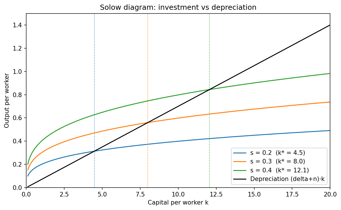

Each coloured curve is the investment schedule for a different savings rate. Where each curve crosses the depreciation line (black) is the corresponding steady state k. Higher savings → higher k, but with diminishing returns: doubling s does not double k*.

What’s Next

• Add technological progress by replacing k^alpha with A(t) · k^alpha where A grows at rate g — the full Solow model.
• Vary delta and n to see their effect on k* — a useful exercise for understanding why rich countries tend to have higher capital per worker.
• Up next: back to biochemistry with the linear-chain Michaelis-Menten model, which showcases mxlpy’s ability to build models programmatically.