Lotka Volterra model
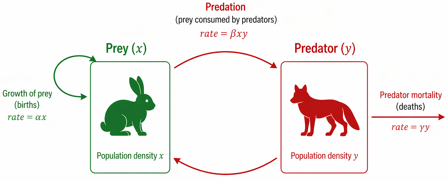
The Lotka-Volterra equations, developed in the 1920s by Alfred Lotka and Vito Volterra representing the cyclic, phase-shifted population dynamics between a predator and its prey.
tune
Simulation parameters
tune
Initial conditions
analytics
Analyses
Short Simulation
Loading chart...
Extended Simulation
Loading chart...
Add analysis
Model Details
Review and edit model structure, biological variables, and kinetic parameters.
| Name | Tex name | Initial value | Actions |
|---|---|---|---|
Edit Options
Edit Options
preview
Generated LaTeX Code
\begin{align*}
  \frac{d Prey}{dt} &= \alpha \cdot Prey - \beta \cdot Predator \cdot Prey \\
  \frac{d Predator}{dt} &= \delta \cdot Predator \cdot Prey - \gamma \cdot Predator
\end{align*}
Fit to data
Fit settings
| Setting | Value |
|---|---|
| Fit backend | |
| Function evaluations per progress update | |
| Maximum total function evaluations | |
| Stop once residual norm reaches |
Curriculum learning (advanced)
Every bar shares one fixed step budget. Drag a divider to move a cutoff, drag a bar's top edge (or focus it and use the arrow keys) to change its share — the final stage isn't draggable, it always gets whatever's left. Double-click a bar or use its + to split it, use a divider's × (or Delete/Backspace while it's focused) to remove it.
Split into equal stages:
min viable
t=0 t=100
| Stage | Data cutoff | Iteration budget |
|---|---|---|
| 1 (final) | full data | 1000 iterations (runs to convergence within this) |
Data
Plot options
| Parameter | Fit | Log-space | Initial guess / fixed value | Fitted value |
|---|---|---|---|---|
| Alpha | — | |||
| Beta | — | |||
| Gamma | — | |||
| Delta | — |
Edit analysis
Plot options
Variable selection
Show Normalize
Edit analysis
Plot options
Variable selection
Show Normalize